Juliaを使ってみる(17/22)：ラプラス近似(その4)

###########################################
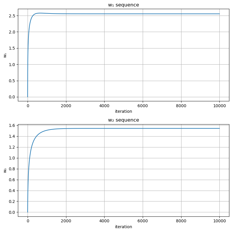
### Laplace近似によるロジスティック回帰 ###
###########################################

using Distributions, PyPlot, ForwardDiff, LinearAlgebra

# n次元単位行列
eye(n) = Diagonal{Forward64}(I, n)

# パラメータ抽出用の関数
unzip(a) = map(x -> getfield(a, x), fieldnames(eltype(a)))

# グラフの諸設定を行う関数
function set_options(ax, xlabel, ylabel, title;
                      grid = true, gridy = false, legend = false)
    ax.set_xlabel(xlabel)
    ax.set_ylabel(ylabel)
    ax.set_title(title)
    if grid
        if gridy
            ax.grid(axis = "y")
        else
            ax.grid()
        end
    end
    legend && ax.legend()
end

# 最適化ラッパー関数の定義
function gradient_method(f, x_init, η, maxiter)
    x_seq = Array{typeof(x_init[1]), 2}(undef,length(x_init), maxiter)
    g(x) = ForwardDiff.gradient(f, x)
    x_seq[:, 1] = x_init
    
    for i in 2:maxiter
        x_seq[:, i] = x_seq[:, i-1] + η*g(x_seq[:, i-1])
    end
    
    x_seq
end


function inference_wrapper_gd(log_joint, params, w₁_init, η, maxiter)
    ulp(w₁) = log_joint(w₁, params...)
    w₁_seq = gradient_method(ulp, w₁_init, η, maxiter)
    w₁_seq
end


### 観測値
X_obs = [-3,1,2]
Y_obs = Bool.([0,1,1])

sig(x) = 1/(1 + exp(-x))

# 事前分布の設定
μ₁ = 0
μ₂ = 0
σ₁ = 10.0
σ₂ = 10.0

# 対数同時分布
log_joint(w, X, Y, μ₁, σ₁, μ₂, σ₂) = 
    logpdf(Normal(μ₁,σ₁), w[1]) +
    logpdf(Normal(μ₂,σ₂), w[2]) +
    sum(logpdf.(Bernoulli.(sig.(w[1]*X_obs .+ w[2])), Y_obs))
params = (X_obs, Y_obs, μ₁, σ₁, μ₂, σ₂)

# 非正規化対数事後分布
ulp(w) = log_joint(w, params...)

### 最適化用パラメータ
w_init = [0.0, 0.0]
maxiter = 10000
η = 0.1

# 最適化の実施
w_seq = inference_wrapper_gd(log_joint, params, w_init, η, maxiter)

# 勾配法の過程を可視化
fig,axes = subplots(2, 1, figsize = (8,8))
axes[1].plot(w_seq[1,:])
set_options(axes[1], "iteration", "w₁", "w₁ sequence")
axes[2].plot(w_seq[2,:])
set_options(axes[2], "iteration", "w₂", "w₂ sequence")

tight_layout()

# 平均
μ_approx = w_seq[:,end]

# 共分散
hessian(w) = ForwardDiff.hessian(ulp, w)
Σ_approx = inv(-hessian(μ_approx))

w₁s = range(-10, 30, length = 1000)
w₂s = range(-20, 20, length = 1000)

fig, axes = subplots(1, 2, figsize = (8,4))
cs = axes[1].contour(w₁s, w₂s, [exp(ulp([w₁,w₂])) + eps() for w₁ in w₁s, w₂ in w₂s]', cmap = "jet")
axes[1].clabel(cs, inline = true)
set_options(axes[1], "w₁", "w₂", "unnormalised posterior")
cs = axes[2].contour(w₁s, w₂s, [pdf(MvNormal(μ_approx, Σ_approx), [w₁,w₂]) for w₁ in w₁s, w₂ in w₂s]', cmap = "jet")
axes[2].clabel(cs, inline = true)
set_options(axes[2], "w₁", "w₂", "approximate posterior")

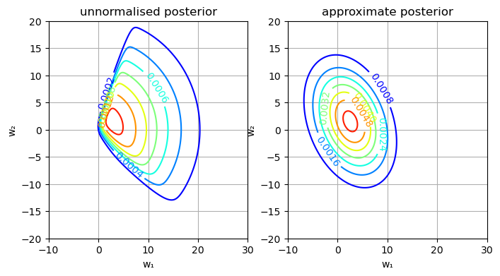
このようにロジスティック回帰では、事後分布が多変量正規分布にならず、近似が上手くいかない。

次回

power-of-awareness.com

今回やりたいこと

前回

1. 勾配を用いる必要性

1.2 勾配を用いた計算の効率化

1.2.4 ロジスティック回帰

次回

1.　勾配を用いる必要性

1.2　勾配を用いた計算の効率化

1.2.4　ロジスティック回帰