以下の書籍

を中心に時系列解析を勉強していきます。
15. 一般状態空間モデルの一括解法
15.4 推定精度向上のためのテクニック
は繰り返し数を無限にした際に理想的な性能を達成することができる。これに対して現実の実装では繰り返し数は有限であるから、その理想的な性能よりも劣化する。そのためより少ない繰り返し数で性能を維持すべく、アルゴリズムから実装に及ぶまで様々な改善手法が提案されている。
15.4.2 実例
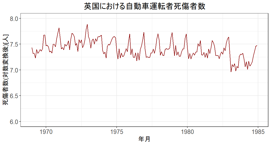
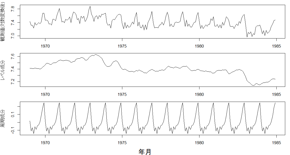
英国における自動車運転者死傷者数について、ローカル・レベル・モデルと周期モデルを用いて分析する。
ここでは、
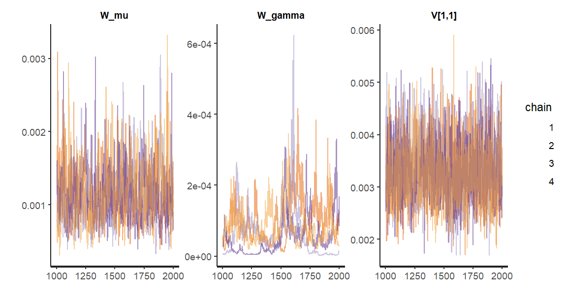
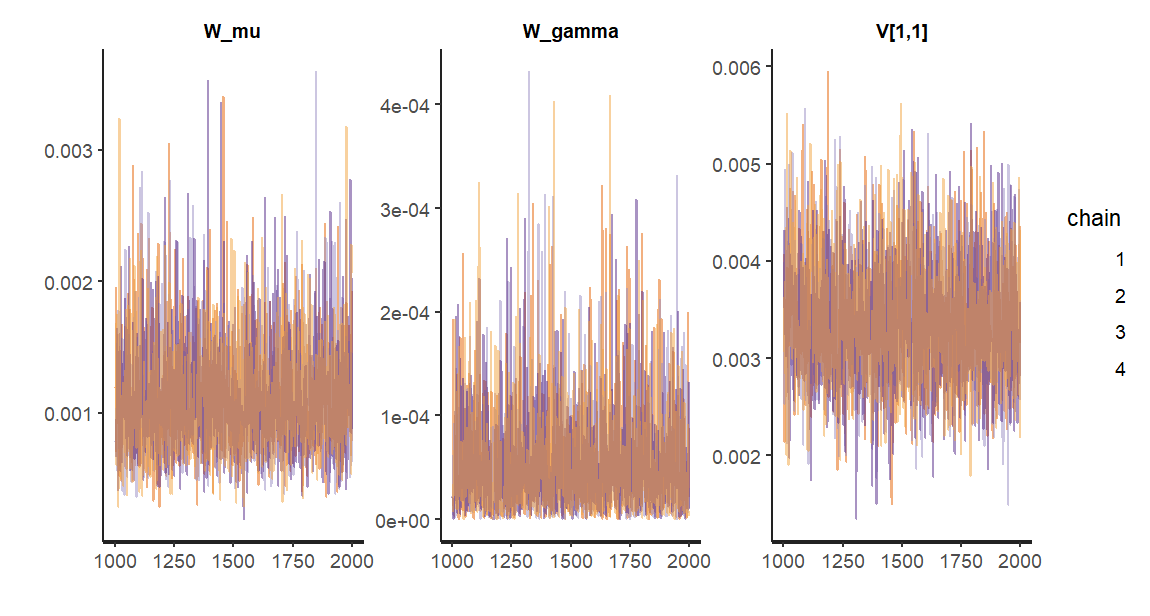
の3パターンを試行する。
########################################################################
### データ分析例                                                     ###
###   英国における自動車運転者死傷者数                               ###
###     (1) 母数を最尤推定し、カルマン平滑化を実施                   ###
###     (2) MCMCで母数も状態もサンプリングする                       ###
###     (3) MCMCで母数のみサンプリングし、FFBSで状態の標本を再生する ###
########################################################################

set.seed(123)

library("dlm")
library("ggplot2")
library("rstan")

# データを対数変換
y <- log(UKDriverDeaths)
t_max <- length(y)

y_for_graph <- data.frame(x = as.numeric(time(y)),y = as.numeric(y))
y_min_max <- c(floor(min(y_for_graph[,"y"])),ceiling(max(y_for_graph[,"y"])))


g <- ggplot(data = y_for_graph, aes(x = x, y = y))
g <- g + geom_area(fill = "salmon", alpha = 0.5,
                   color= "darkred", outline.type = "upper")
g <- g + theme_bw()
g <- g + labs(title = "英国における自動車運転者死傷者数",
              x = "年月",y = "死傷者数(対数変換後)[人]")
g <- g + coord_cartesian(ylim = y_min_max)
g <- g + theme(axis.text= element_text(size = 12),
               axis.text.x=element_text(size = 12),
               legend.title = element_blank(),
               legend.text = element_text(size = 12),
               legend.position = "top",
               axis.title = element_text(size = 12),
               axis.title.y = element_text(angle = 90,size = 12),
               plot.title= element_text(size = 16,hjust = 0.5))
plot(g)


# モデルのテンプレート
mod <- dlmModPoly(order = 1) + dlmModSeas(frequency = 12)

# モデルを定義・構築するユーザ定義関数
build_dlm_UKD <- function(par){
  mod$W[1,1] <- exp(par[1])
  mod$W[2,2] <- exp(par[2])
  mod$V[1,1] <- exp(par[3])

  return(mod)
}

# 母数の最尤推定
fit_dlm_UKD <- dlmMLE(y = y, parm = rep(0, times = 3), build = build_dlm_UKD)

# モデルの設定と結果の確認
mod <- build_dlm_UKD(fit_dlm_UKD$par)
cat(diag(mod$W)[1:2], mod$V, "\n")

# 平滑化処理
dlmSmoothed_obj <- dlmSmooth(y = y, mod = mod)

   mu <- dropFirst(dlmSmoothed_obj$s[,1])
gamma <- dropFirst(dlmSmoothed_obj$s[,2])

# 結果のプロット
oldpar <- par(no.readonly = T)
par(mfrow = c(3,1))
par(oma = c(2,0,0,0))
par(mar = c(2,4,1,1))
ts.plot(    y, ylab = "観測値(対数変換後)")
ts.plot(   mu, ylab = "レベル成分")
ts.plot(gamma, ylab = "周期成分")
mtext(text = "年月", side = 1, line = 1, outer = T)
par(oldpar)

########################

#### Stanを用いた事後同時分布からの標本取得

# まずは状態も含めてサンプリングする

# Stanの事前設定
rstan_options(auto_write = T)
options(mc.cores = parallel::detectCores())
theme_set(theme_get() + theme(aspect.ratio = 3/4))

# モデル:生成、コンパイル
stan_mod_out <- stan_model(file = "C:/Users/Julie/Desktop/model10-4.stan")

# 平滑化:実行(サンプリング)
fit_stan <- sampling(object = stan_mod_out,
                     data = list(t_max = t_max, y = y, m0 = mod$m0, C0 = mod$C0),
                     pars = c("W_mu", "W_gamma", "V"),
                     seed = 123
                     )
fit_stan

traceplot(fit_stan, pars = c("W_mu", "W_gamma", "V"), alpha = 0.5)

########################

#### Stanを用いた事後同時分布からの標本取得
# モデル:規定(ローカル・レベル・モデル+周期モデル(時間領域アプローチ),カルマンフィルタを利用)

# 状態を含めずにサンプリングする

# Stanの事前設定
rstan_options(auto_write = T)
options(mc.cores = parallel::detectCores())
theme_set(theme_get() + theme(aspect.ratio = 3/4))

# モデル:生成、コンパイル
stan_mod_out <- stan_model(file = "C:/Users/Julie/Desktop/model10-5.stan")

# 平滑化:実行(サンプリング)
fit_stan <- sampling(object = stan_mod_out,
                     data = list(t_max = t_max, y = matrix(y, nrow = 1),
                                 G = mod$G,
                                 F = t(mod$F),
                                 m0 = mod$m0, C0 = mod$C0),
                     pars = c("W_mu", "W_gamma", "V"),
                     seed = 123
)

fit_stan

traceplot(fit_stan, pars = c("W_mu", "W_gamma", "V"), alpha = 0.5)

cat(summary(fit_stan)$summary["W_mu","mean"],
    summary(fit_stan)$summary["W_gamma","mean"],
    summary(fit_stan)$summary["V[1,1]","mean"],"\n")


#### FFBSで状態を再現
stan_mcmc_out <- rstan::extract(fit_stan, pars = c("W_mu", "W_gamma", "V"))

# FFBSの前処理
it_seq <- seq_along(stan_mcmc_out$V[,1,1])
progress_bar <- txtProgressBar(min = 1, max = max(it_seq), style = 3)

x_FFBS <- lapply(it_seq, function(it){
  # 進捗バーの表示
  setTxtProgressBar(pb = progress_bar, value = it)

  # W,Vの値をモデルに設定
  mod$W[1,1] <- stan_mcmc_out$W_mu[it]
  mod$W[2,2] <- stan_mcmc_out$W_gamma[it]
  mod$V[1,1] <- stan_mcmc_out$V[it,1,1]

  # FFBSの実行
  return(dlmBSample(dlmFilter(y = y, mod = mod)))
})

# FFBSの後処理
x_mu_FFBS <- t(sapply(x_FFBS, function(x){x[-1,1]}))
x_gamma_FFBS <- t(sapply(x_FFBS, function(x){x[-1,2]}))

mu_FFBS <- colMeans(x_mu_FFBS)
gamma_FFBS <- colMeans(x_gamma_FFBS)