Juliaを基礎からゆっくりと（その14/18）

　や、言語関係など覚えたいもの、覚えるべきものはたくさんある一方で、注目が集まっているから、やってみたい。ということでプログラミング言語としてのを学んでいく。

1から始める Juliaプログラミング

前回

power-of-awareness.com

3.　Juliaライブラリの使い方

3.5　可視化

##########################
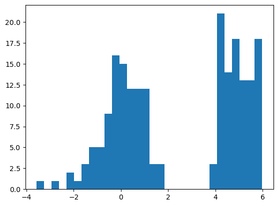
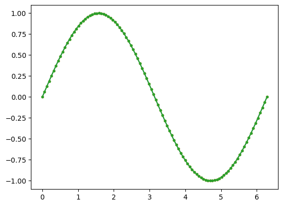
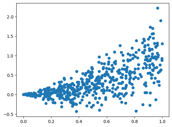
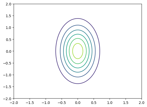
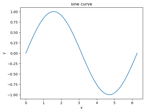
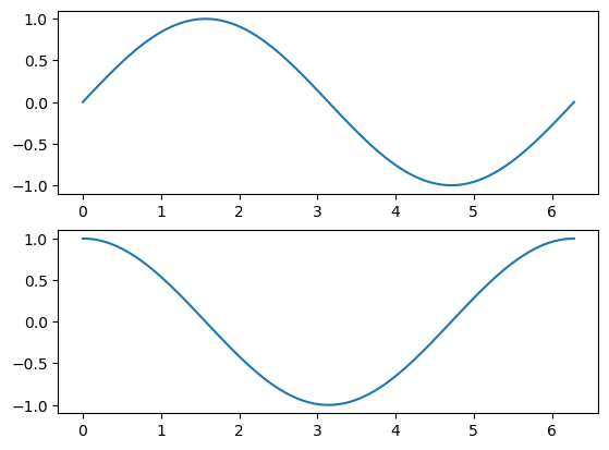
### PyPlotによる可視化 ###
##########################

using PyPlot
using Distributions

# ヒストグラム
x = vcat(randn(100), 2 * rand(100) .+ 4)

hist(x, bins = 30)

# グラフ
y = range(0, 2pi, length = 100)

plot(y, sin.(y))
plot(y, sin.(y), ".") # 点マーカーのみ
plot(y, sin.(y), ".-") # マーカーと線の両方を出力
# savefig("name.png") # 図を保存

# 散布図
x = rand(500)
y = x .^2 + randn(500) .* abs.(x) * 0.5

scatter(x,y)

# 等高線
f(x,y) = exp(-(x^2+4y^2))

x = y = range(-2,2,length=100)

f.(x, y') == [f(xx, yy) for xx in x, yy in y] 

contour(x, y, f.(x,y'))

# グラフの編集
z = range(0, 2pi, length = 100)

plot(z, sin.(z))
title("sine curve")
xlabel("x")
ylabel("y")

# サブプロット
x = range(0, 2pi, length = 100)

for i in 1:2
    subplot(2,1,i)
    
    if i ==1
        plot(x, sin.(x))
    else
        plot(x, cos.(x))
    end
end

3.5.1　オブジェクト指向インターフェース

　使い方はと同様である。

########################################
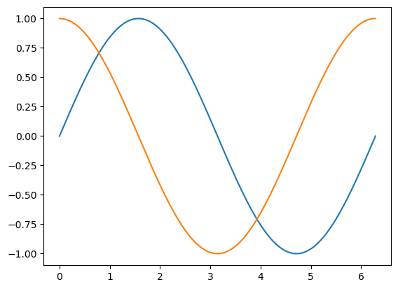
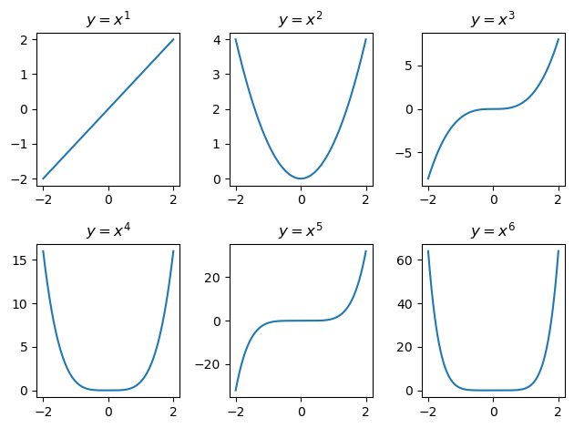
### オブジェクト指向インターフェース ###
########################################

fig, ax = subplots()

x = range(0,2pi, length = 1000)

ax.plot(x, sin.(x))
ax.plot(x, cos.(x))

fig, axes = subplots(2,3)

x = range(-2, 2, length = 1000)

for i in 1:2, j in 1:3
    ax = axes[i,j]
    ax.plot(x, x.^(3(i-1)+j))
    ax.set_title("\$y = x^$(3(i-1)+j)\$")
end

fig.tight_layout()

次回

power-of-awareness.com