")
1. ロジスティック回帰
ロジスティック回帰は2値を取り得るため、まずはその2値を表現するのに分布を用いることにする。その
分布の確率パラメータ
の定式化を次に考える。ここでは
としたいが、そうすると実数全体を取り得るため、シグモイド関数を用いることとする。すなわち
で与えられる。
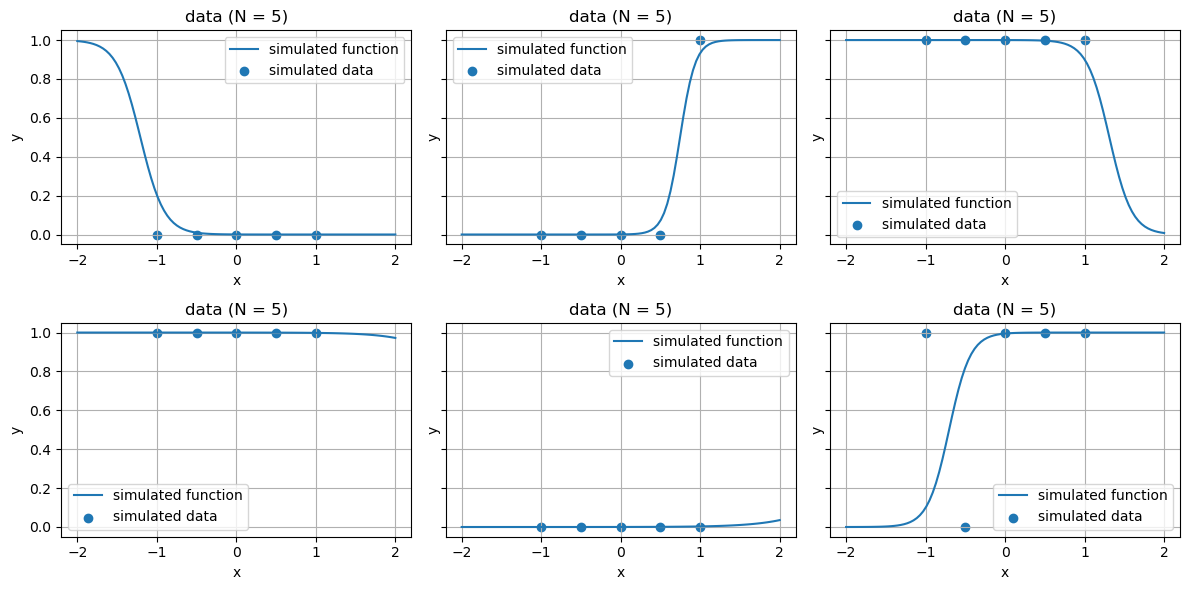
##########################
### ロジスティック回帰 ###
##########################

using Distributions
using PyPlot

# グラフの諸設定を行う関数
function set_options(ax, xlabel, ylabel, title;
                      grid = true, gridy = false, legend = false)
    ax.set_xlabel(xlabel)
    ax.set_ylabel(ylabel)
    ax.set_title(title)
    if grid
        if gridy
            ax.grid(axis = "y")
        else
            ax.grid()
        end
    end
    legend && ax.legend()
end


###
sig(x)= 1/(1+exp(-x))

# パラメータ、関数、出力集合Yを生成
function generate_logistic(X, μ₁,μ₂,σ₁,σ₂)
    w₁ = rand(Normal(μ₁,σ₁))
    w₂ = rand(Normal(μ₂,σ₂))

    f(x) = sig(w₁*x+w₂)
    Y = rand.(Bernoulli.(f.(X)))

    Y, f, w₁, w₂
end

# パラメータ
μ₁ = 0
μ₂ = 0
σ₁ = 10.0
σ₂ = 10.0
X = [-1.0,-0.5,0,0.5,1.0]

xs = range(-2, 2, length = 100)

fig, axes = subplots(2, 3, sharey = true, figsize = (12,6))
for ax in axes
    # 関数f,出力Yの生成
    Y, f, w₁, w₂ = generate_logistic(X,μ₁,μ₂,σ₁,σ₂)

    # 生成された直線とYのプロット
    ax.plot(xs, f.(xs), label = "simulated function")
    ax.scatter(X, Y, label = "simulated data")

    set_options(ax, "x", "y", "data (N = $(length(X)))", legend = true)
end

tight_layout()
2.1 伝承サンプリング
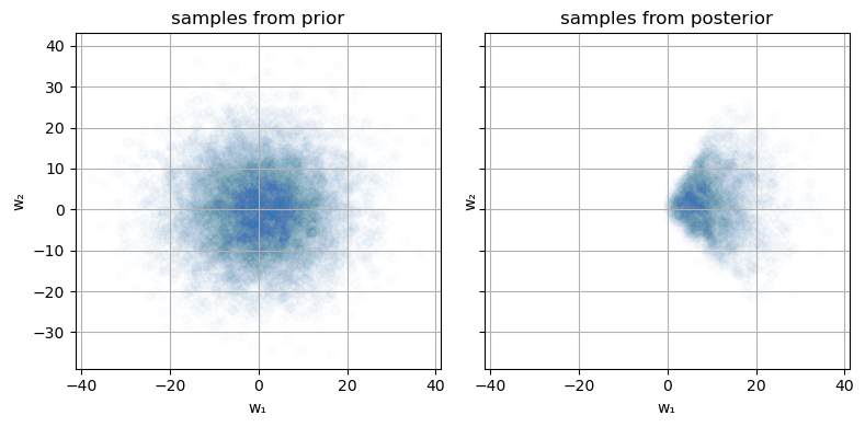
######################################
### 伝承サンプリングによる事後分布 ###
######################################

### 観測データ
X_obs = [-2,1,2]
Y_obs = Bool.([0, 1, 1])

fig,ax = subplots()
ax.scatter(X_obs, Y_obs)
ax.set_xlim([-3,3])

set_options(ax, "x", "y", "data (N = $(length(X_obs)))")

### 事後分布
# 最大サンプリング数
maxiter = 10_000

# パラメータ(保存用)
param_posterior = Vector{Tuple{Float64, Float64}}()

for i in 1:maxiter
    # 関数f,出力Yの生成
    Y, f, w₁, w₂ = generate_logistic(X_obs, μ₁, μ₂, σ₁, σ₂)

    # 観測データと一致していれば、そのときのパラメータwを保存
    Y == Y_obs && push!(param_posterior, (w₁,w₂))
end

# 標本受容率
acceptance_rate = length(param_posterior) / maxiter
println("acceptance rate = $(acceptance_rate)")


# パラメータ抽出用の関数
unzip(a) = map(x -> getfield.(a, x), fieldnames(eltype(a)))

# 事前分布からのサンプル
param_prior = [generate_logistic(X, μ₁, μ₂, σ₁,σ₂)[3:4] for i in 1:10_000]
w₁_prior, w₂_prior = unzip(param_prior)

# 事後分布からのサンプル
w₁_posterior, w₂_posterior = unzip(param_posterior)

fig, axes = subplots(1, 2, sharex = true, sharey = true, figsize = (8, 4))

# 事前分布
axes[1].scatter(w₁_prior,w₂_prior, alpha = 0.01)
set_options(axes[1], "w₁", "w₂", "samples from prior")

# 事後分布
axes[2].scatter(w₁_posterior,w₂_posterior, alpha = 0.01)
set_options(axes[2], "w₁", "w₂", "samples from posterior")

tight_layout()
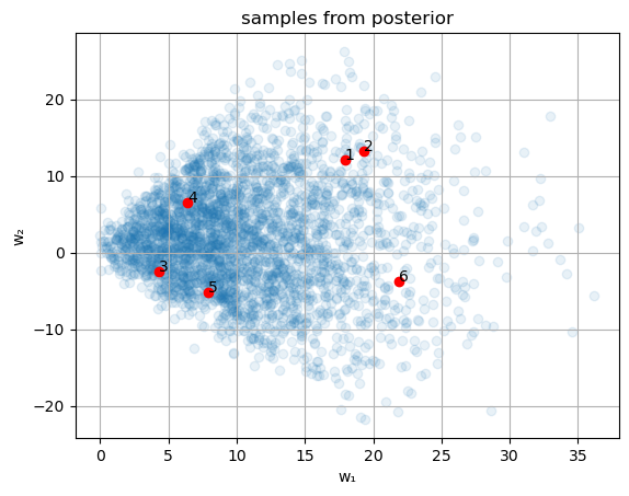
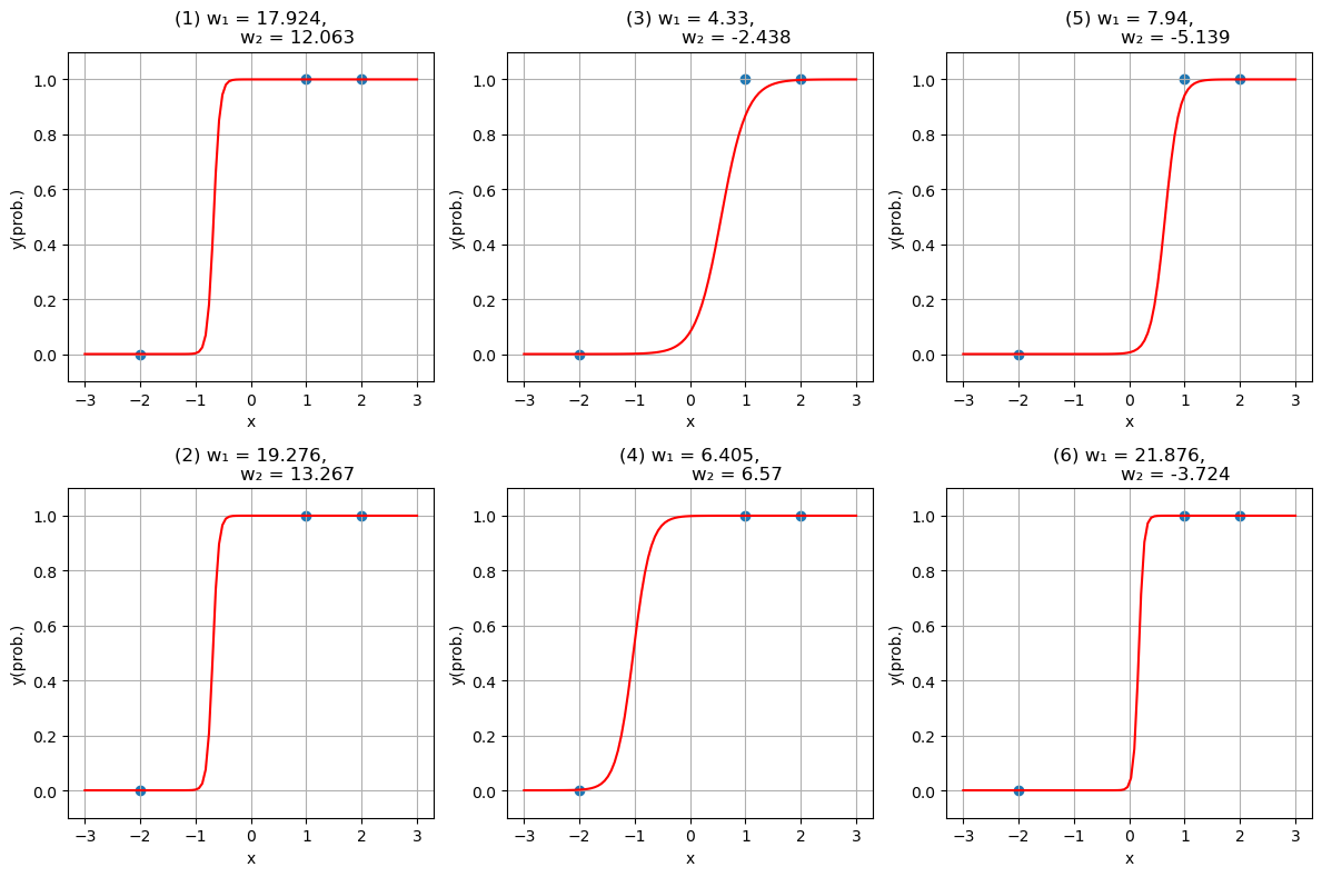
# 関数を可視化する範囲
xs = range(-3, 3, length = 100)

# サンプリングで得られたパラメータ全体のプロット
fig, ax = subplots()
ax.scatter(w₁_posterior, w₂_posterior, alpha = 0.1)
set_options(ax, "w₁", "w₂", "samples from posterior")


fig,axes = subplots(2, 3, figsize = (12, 8))
for i in eachindex(axes)
   # 関数を可視化するためのwを取得
    j = round(Int, length(param_posterior) * rand()) + 1
    w₁,w₂ = param_posterior[j]

    # 選択されたw
    ax.scatter(w₁, w₂, color = "r")
    ax.text(w₁, w₂, i)

    # 対応する関数のプロット
    f(x) = sig(w₁ * x + w₂)
    axes[i].plot(xs, f.(xs), "r")

    # 観測データのプロット
    axes[i].scatter(X_obs, Y_obs)

    axes[i].set_ylim([-0.1, 1.1])
    set_options(axes[i], "x", "y(prob.)",
        "($(i)) w₁ = $(round(w₁, digits = 3)),
                w₂ = $(round(w₂, digits = 3))")
end
tight_layout()
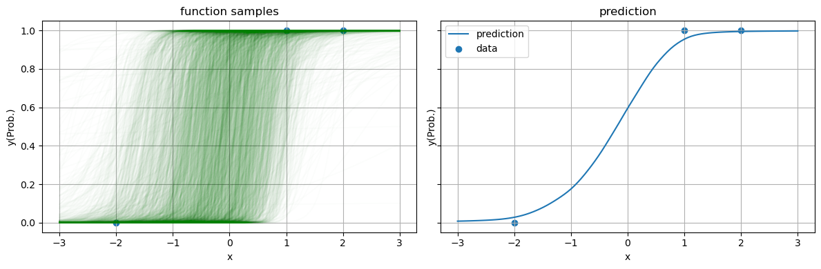
2.2 予測分布のプロット
fig, axes = subplots(1, 2, sharey = true, figsize = (12, 4))

fs = []
for (i, param) in enumerate(param_posterior)
    # 1サンプル分のパラメータ
    w₁, w₂ = param

    # 1サンプル分の予測関数
    f(x) = sig(w₁ * x + w₂)
    axes[1].plot(xs, f.(xs), "g", alpha = 0.01)

    push!(fs, f.(xs))
end

axes[1].scatter(X_obs, Y_obs)
set_options(axes[1], "x", "y(Prob.)", "function samples")

# 予測確率
axes[2].plot(xs, mean(fs), label = "prediction")
axes[2].scatter(X_obs, Y_obs, label = "data")
set_options(axes[2], "x", "y(Prob.)", "prediction", legend = true)

tight_layout()
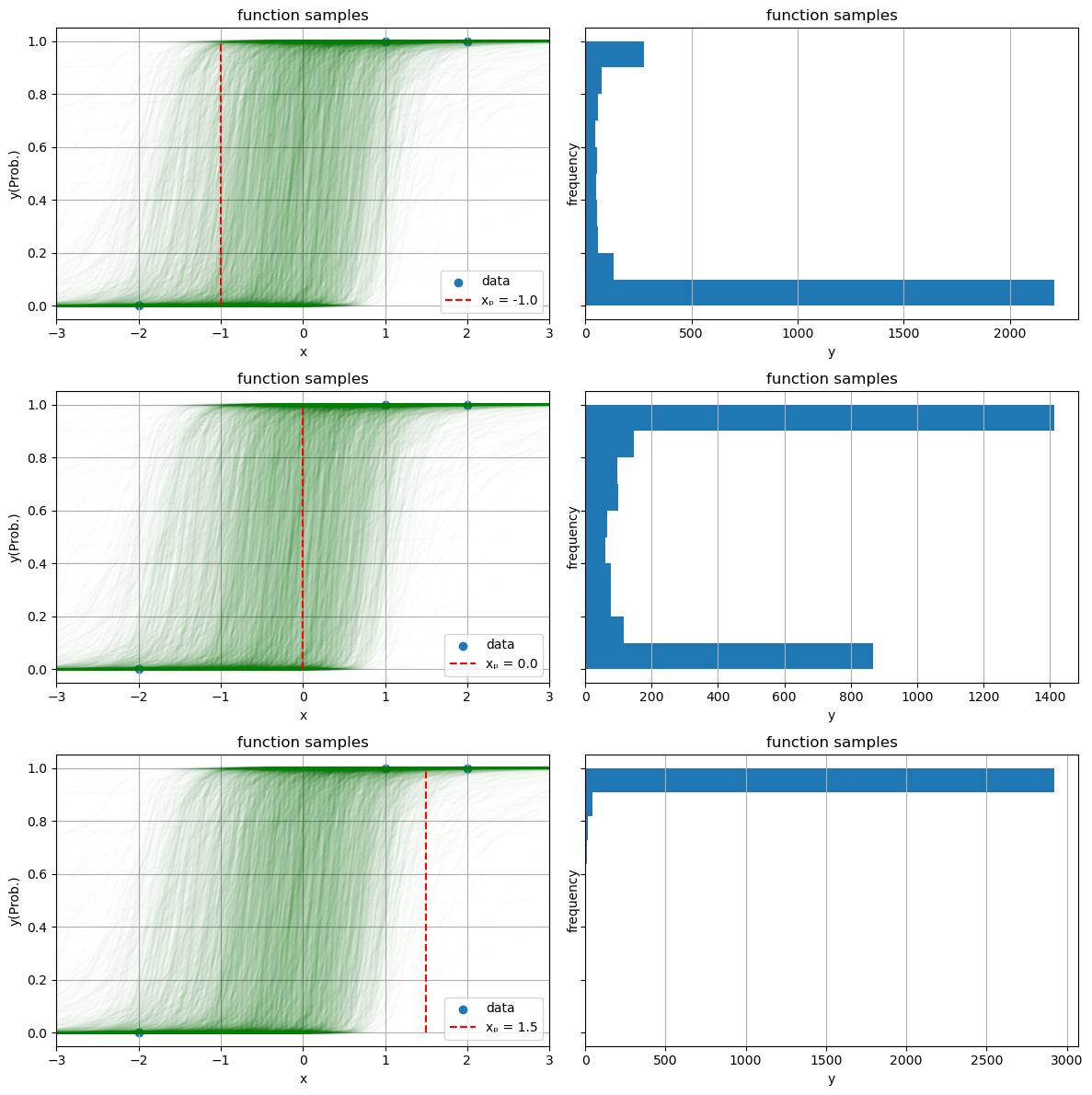
2.3 特定の点の予測値
# 予測対象の点候補
x_list = [-1.0, 0.0, 1.5]

fig_num = length(x_list)
fig,axes = subplots(fig_num, 2, sharey = true, figsize = (12, 4 * fig_num))
for (j, x) in enumerate(x_list)
    # パラメータごとに関数を可視化
    for (i, param) in enumerate(param_posterior)
        w₁, w₂ = param
        f(x) = sig(w₁*x+w₂)
        axes[j].plot(xs, f.(xs), "g", alpha = 0.01)
    end

    # 観測値
    axes[j].scatter(X_obs, Y_obs, label = "data")

    # 候補点のx座標
    axes[j].plot([x,x],[0,1], "r--", label = "xₚ = $(x)")

    axes[j].set_xlim(extrema(xs))
    set_options(axes[j], "x", "y(Prob.)", "function samples")
    axes[j].legend(loc = "lower right")

    # 点xにおける関数値をヒストグラムとして可視化
    probs = [sig(param[1] * x + param[2]) for param in param_posterior]
    axes[j + fig_num].hist(probs, orientation = "horizontal")
    set_options(axes[j + fig_num], "y", "frequency", "function samples", grid = false)
    axes[j + fig_num].grid(axis = "x")
end

tight_layout()