はじめに
さまざまなテキスト

")
などを参照しながらベイズ統計学について学んでいきます。
また理論だけでなく、可能な限りシミュレーションを含めていくこととし、それも,
や
など幅広い言語で実装していきたい。
各種バージョン情報
今回のまとめ
3. Bayes推定
3.6 Bayes推定の実例:Bernoulli試行
企業の信用力を評価すべく、納期に遅れる確率を考えることとし、納期に遅れる確率をと書くことにする。
3.6.1 逐次的にデータを活用した場合
ある企業との取引について、番目の取引について納期通りに納品された場合には
、納期に遅れた場合には
を取るような確率変数
と定義する。
このとき、の確率分布は
である。
このとき、納期の遅れのパターンからある企業社が納期に遅れる確率を
統計学に基づいて推測する。
まず社が1回目の納期に遅れたときの納期に遅れる確率
の推測を考える。
の定理より
が成り立つ。
について無情報事前分布を用いることとすれば、
であり、またであるとき、
である。更に
に注意すれば、
が成り立つ。
次に2回目の納期にも遅れたと仮定する。このときの事後分布のカーネルは
の定理から
である。またであるから、
以上、帰納的にの定理を適用することで
回続けて納期を遅れたという状況での
の事後分布は
である。
3.6.2 一括でデータを活用した場合
前節では逐次的にデータを用いて事後分布を導出したが、次に過去の納期に関する情報をまとめて使っての事後分布を導出する。
たとえば過去5回の納期に関するデータとして
を得たとしよう。
は互いに独立であるから、
であり、具体的にが与えられていることから
である。の関数と見るとき、これを尤度という。
の定理から
が成り立つ。
一般の場合として納期を回の場合を考える。
ここでと定義すると
である。
の定理より
が成り立つ。ここではベータ関数である。これはベータ分布である。すなわち
である。
3.7 信用集合
信用集合()は事後分布の不確実性を伝える有効な手法の1つである。
母数空間をとする。実数
に対して
を満たすようなを確率
の信用集合(確信集合)という。特に
が区間であれば、信用区間・確信区間(
)という。
しかし定義からでは、信用集合は一意に決まらない。たとえば
を満たすような実数を選び、
とする等裾事後信用区間(
-
)や、その区間内の確率密度が必ず区間外の密度よりも大きくなる最高事後密度区間(
区間)、すなわち
に対して
を満たすような区間を採用することが多い。
区間は母数の真の値がそこに含まれる確率密度が低いような区間を含まなくなることから、母数の真の値である蓋然性がより高い区間を含み得るという点で、等裾事後信用区間よりも優れていると言える。
伝統的な統計学でいう信頼区間に対応するのが等裾事後信用区間である。信頼区間は、ある分析において何度も推定値および信頼区間を計算したときに、推定値がその信頼区間に収まる頻度がであることを意味する。これに対して、信用区間は想定した確率モデルの母数がその区間に含まれる確率が
であることを意味する。
3.8 Bayes統計学における仮説検定
統計学における仮説検定
は、パラメータの事後分布
において仮説
が成り立つ事後確率
を評価する。その仮説の事後確率が
に近ければその仮説は正しいと評価してもよかろう。
統計学における2つの仮説に対する仮説検定*1
では、
を
で定義する。最右辺の除数を事前オッズ比、被除数を事後オッズ比という。事前オッズ比も事後オッズ比もが小さければ分母の対立仮説
が分子の帰無仮説
よりも正しい確率が大きいことを意味する。したがって
- 事前オッズ比は事前情報において対立仮説
が帰無仮説
に対してどれだけ蓋然性の高さで優位にあるかを意味する。
- 事後オッズ比は情報
が加わったことを考慮した対立仮説
であり、はデータ
が加わったことで対立仮説
の帰無仮説
に対する蓋然性の高さの観点での優位性がどれだけ変わったかを意味する。
とはいえは事前情報にも依存している。事後確率は
であるから、事後オッズ比について
が成り立つ。したがって
であり、このようにの評価には事前分布
が加味されている。
3.9 将来予測と意思決定
分析における予測の方法を考える。すなわちデータ
を観測して事後分布が分かっているとして、未観測の実現値を
とすれば、その分布は未知の値である
のデータ
が観測されたという条件の下での条件付確率分布
を考え、これを予測分布という。ここで
であるから、
が成り立つ。
実際には、将来データの予測値を得るべく上記の予測分布を用いたり、事前分布の観測データに対する適合度を得るべく周辺尤度
を利用したりする。
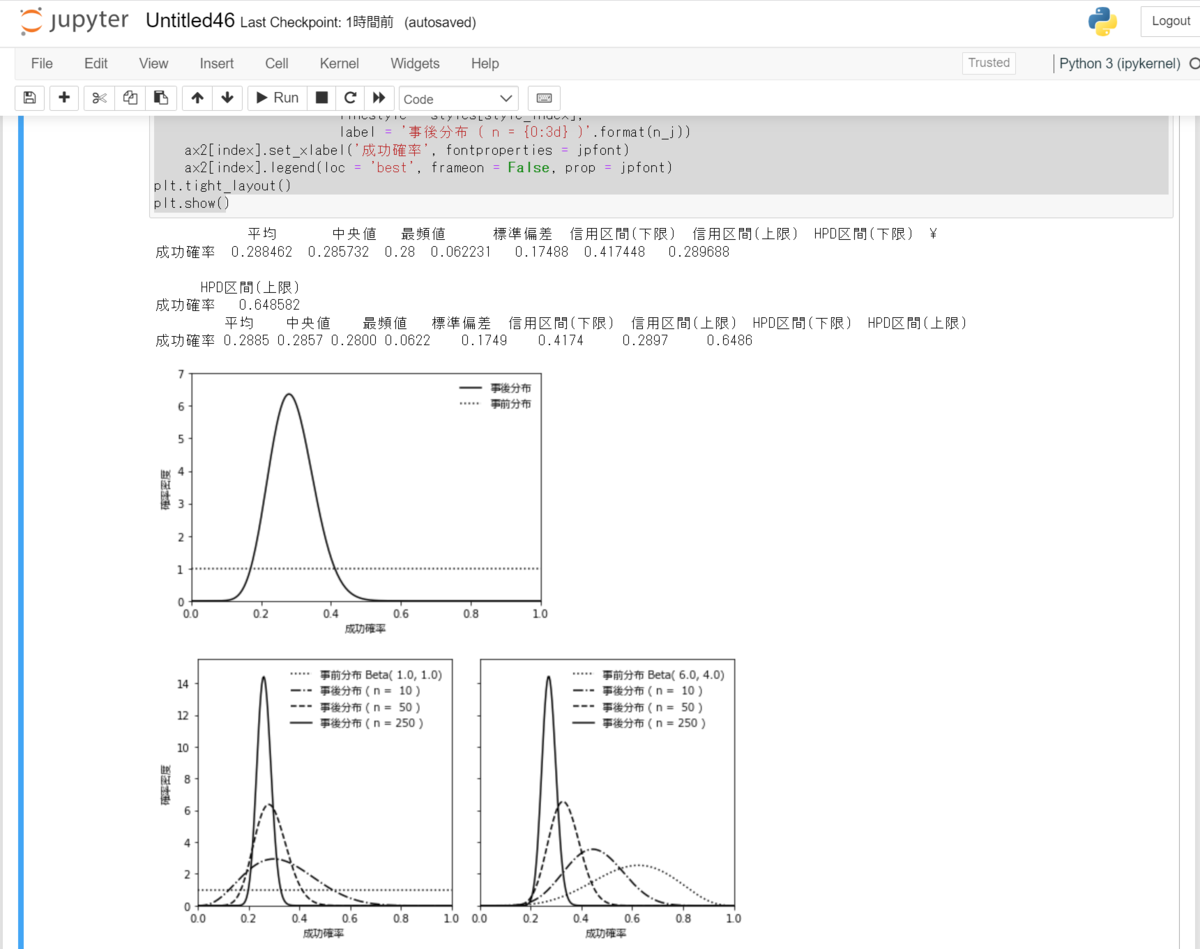
3.10 Pythonでの実装例
中妻(2019) PP. 37-40を基にした。
##################
### ベイズ推論 ###
##################

import numpy as np
import scipy.stats as st
import scipy.optimize as opt
import pandas as pd
import matplotlib.pyplot as plt
from matplotlib.font_manager import FontProperties
import sys

FontPath = r'C:\\Windows\Fonts\meiryo.ttc'

jpfont = FontProperties(fname = FontPath)

###
### Bernoulli分布のHPD区間の計算

def beta_hpdi(ci0, alpha, beta, prob):
    def hpdi_conditions(v, a, b, p):
        eq1 = st.beta.cdf(v[1], a, b) - st.beta.cdf(v[0], a, b) - p
        eq2 = st.beta.cdf(v[1], a, b) - st.beta.cdf(v[0], a, b)
        return np.hstack((eq1, eq2))
    return opt.root(hpdi_conditions, ci0, args = (alpha, beta, prob)).x
def bernoulli_stats(data, a0, b0, prob):
    n = data.size
    sum_data = data.sum()
    a = sum_data + a0
    b = n - sum_data + b0
    mean_pi = st.beta.mean(a, b)
    median_pi = st.beta.median(a, b)
    mode_pi = (a - 1.0) / (a + b - 2.0)
    sd_pi = st.beta.std(a, b)
    ci_pi = st.beta.interval(prob, a, b)
    hpdi_pi = beta_hpdi(ci_pi, a, b, prob)
    stats = np.hstack((mean_pi, median_pi, mode_pi, sd_pi, ci_pi, hpdi_pi))
    stats = stats.reshape((1,8))
    stats_string = ['平均', '中央値','最頻値','標準偏差','信用区間(下限)','信用区間(上限)',
                    'HPD区間(下限)', 'HPD区間(上限)']
    param_string = ['成功確率']
    results = pd.DataFrame(stats, index = param_string, columns = stats_string)
    return results, a, b

###

p = 0.25
n = 50
np.random.seed(99)
data = st.bernoulli.rvs(p, size = n)

a0 = 1.0
b0 = 1.0
prob = 0.95

results, a, b = bernoulli_stats(data, a0, b0, prob)
print(results)
print(results.to_string(float_format = '{:,.4f}'.format))

# 事後分布のグラフ
fig1 = plt.figure(num = 1, facecolor = 'w')
q = np.linspace(0, 1, 250)
plt.plot(q, st.beta.pdf(q, a, b), 'k-', label = '事後分布')
plt.plot(q, st.beta.pdf(q, a0, b0), 'k:', label = '事前分布')
plt.xlim(0, 1)
plt.ylim(0, 7)
plt.xlabel('成功確率', fontproperties = jpfont)
plt.ylabel('確率密度', fontproperties = jpfont)
plt.legend(loc = 'best', frameon = False, prop = jpfont)
plt.show()

# 事前分布とデータの累積が事後分布の形状に与える影響の可視化
np.random.seed(99)
data = st.bernoulli.rvs(p, size = 250)
value_size = np.array([10, 50, 250])
value_a0 = np.array([1.0, 6.0])

value_b0 = np.array([1.0, 4.0])
styles = [':', '-.', '--', '-']
fig2, ax2 = plt.subplots(1, 2, sharey = 'all', sharex = 'all', num = 2, figsize = (8, 4), facecolor = 'w')

ax2[0].set_xlim(0, 1)
ax2[0].set_ylim(0, 15.5)
ax2[0].set_ylabel('確率密度', fontproperties = jpfont)

for index in range(2):
    style_index = 0
    a0_i = value_a0[index]
    b0_i = value_b0[index]
    ax2[index].plot(q, st.beta.pdf(q, a0_i, b0_i), color = 'k',
                    linestyle = styles[style_index],
                    label = '事前分布 Beta({0: < 3.1f}, {1:<3.1f})'.format(a0_i, b0_i))
    for n_j in value_size:
        style_index += 1
        sum_data = np.sum(data[:n_j])
        a_j = sum_data + a0_i
        b_j = n_j - sum_data + b0_i
        ax2[index].plot(q, st.beta.pdf(q, a_j, b_j), color = 'k',
                        linestyle = styles[style_index],
                        label = '事後分布 ( n = {0:3d} )'.format(n_j))
    ax2[index].set_xlabel('成功確率', fontproperties = jpfont)
    ax2[index].legend(loc = 'best', frameon = False, prop = jpfont)
plt.tight_layout()
plt.show()
参考文献
- 安道知寛(2010)「ベイズ統計モデリング」(朝倉書店)
- 鎌谷研吾・著 駒木文保・編(2020)「モンテカルロ統計計算」(講談社サイエンティフィック)
- 豊田秀樹・編著(2015)「基礎からのベイズ統計学」(朝倉書店)
- 中妻照雄(2007)「入門 ベイズ統計学」(朝倉書店)
- 中妻照雄(2013)「実践 ベイズ統計学」(朝倉書店)
- 中妻照雄(2019)「実践 Pythonライブラリー Pythonによる ベイズ統計学入門」(朝倉書店)
- 馬場真哉(2019)「RとStanではじめるベイズ統計モデリングによるデータ分析入門」(講談社サイエンティフィック)
- 松浦健太郎(2016)「StanとRでベイズ統計モデリング」(共立出版)
- 渡辺澄夫(2012)「ベイズ統計の理論と方法」(コロナ社)
- Andrew Gelman, John Carlin, Hal Stern, David Dunson, Aki Vehtari, and Donald Rubin (2014) "Bayesian Data Analysis", CRC Press
*1:と仮定する。